The very concrete principle of how a cache works

A hash table implemented in hardware 2019.03.30

KO | EN

Principle of Locality
Caches
Cache Metrics
Cache Organization
Associative Cache
- Set Associative Cache Organization
- Concrete Example
Handling Cache Writes
Software Restructuring
References

As technology has advanced, processor speed has risen quickly, but memory speed hasn’t kept up. No matter how fast a processor is, if memory responds slowly the whole system ends up slow. The device that addresses this is the cache.

A cache is a small, fast memory that sits inside the CPU chip. (It’s also expensive.) Going to main memory for data every time is slow, so the cache holds frequently used data and lets the processor reach that data from the cache instead of main memory, which speeds things up.

Principle of Locality

The judgment about which data is “frequently used” follows the principle of locality, which can be split into temporal locality and spatial locality.

Temporal locality is the tendency to access recently accessed data again. For example, the variable i that serves as the index in a loop is accessed several times within a short span.

for (i = 0; i < 10; i += 1) {
  arr[i] = i;
}

Spatial locality is the tendency to access the space near recently accessed data again. In the loop above, as it references each element of the array arr, it accesses nearby memory locations one after another. That’s because an array’s elements are allocated consecutively in memory.

Even within a single process, some parts are used often and others aren’t, so the operating system manages a process by dividing it into units called pages, and the figure above is a trace of page references. The horizontal axis is execution time, and the vertical axis is the memory address. A horizontal run of references means the same memory address was referenced over a long stretch of time, while a vertical run means closely spaced memory addresses were referenced at the same time. You can see that the principle of locality applies to page access too.

Caches

A CPU chip contains several caches, and each one has its own purpose and role.

+-------------+------+------+     +---------------+     +--------+
|             |  I$  |      | <-- |               | <-- |        |
+  Processor  +------+  L2  |     |  Main Memory  |     |  Disk  |
|             |  D$  |      | --> |               | --> |        |
+-------------+------+------+     +---------------+     +--------+

L1 Cache: The cache closest to the processor. For speed, it’s split into I$ and D$.
- Instruction Cache (I$): The cache that handles data in the memory’s TEXT segment.
- Data Cache (D$): The cache that handles all data except the TEXT segment.
L2 Cache: A larger-capacity cache. For the sake of size, it isn’t split the way the L1 cache is.
L3 Cache: The cache shared by multiple cores in a multi-core system.

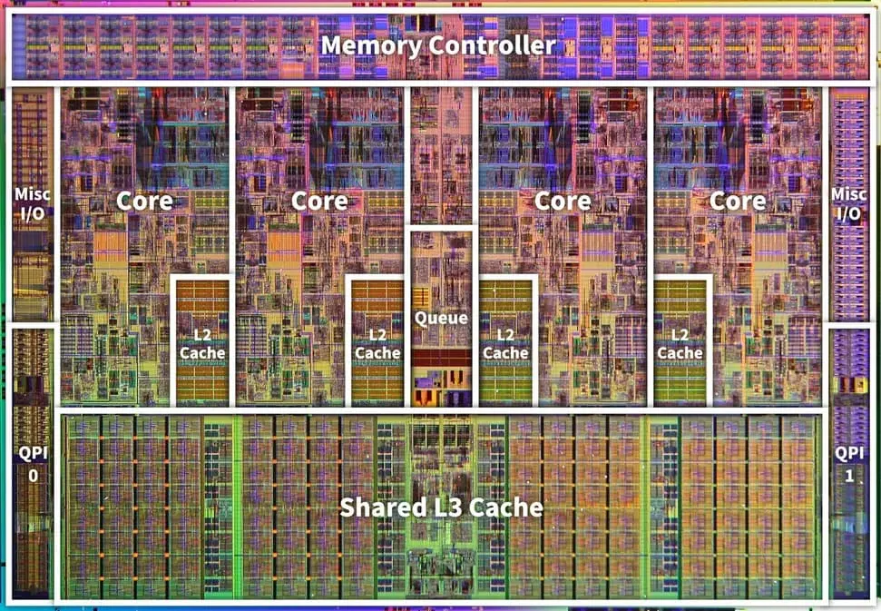
The reason a dollar sign ($) is used for caches is that “cache” is pronounced the same as “cash,” the word for money 😃

A die map of the Intel Core i7 quad-core chip.

Today, caches take up 30 to 70% of a CPU chip’s area. The i486, a single-core processor made in 1989, had just one 8KB I/D cache. The die map of the Intel Core i7 quad-core chip, on the other hand, shows that each of the four cores has its own 256KB L2 cache, plus an 8MB L3 cache shared by all the cores. (The region above the L2 cache looks like the L1 cache, but I wasn’t sure, so I didn’t label it.)

Cache Metrics

When measuring a cache’s performance, hit latency and miss latency are considered important factors.

When the data the CPU requests is in the cache, that’s a cache hit. Hit latency is the time it takes to fetch the cached data on a hit. When the requested data isn’t in the cache, that’s a cache miss, and miss latency is the time it takes to fetch the data from a higher-level cache (for example, when the data isn’t in the L1 cache and is looked up in the L2 cache) or from memory on a miss.

Average access time is calculated as follows:

\begin{aligned} \text{Miss rate} &= {\text{Cache misses} \over \text{Cache acesses}} \\ \text{Average access time} &= \text{Hit latency} + \text{Miss rate} \times \text{Miss latency} \end{aligned}

To improve a cache’s performance, you can shrink the cache to reduce hit latency, enlarge the cache to reduce the miss rate, or use a faster cache to reduce latency.

Cache Organization

A cache is made of fast-responding SRAM (Static Random Access Memory); given an address as a key, it can access the corresponding location immediately. DRAM (Dynamic Random Access Memory) has this same property, but by hardware design DRAM is slower than SRAM. When people say “main memory,” they usually mean DRAM.

Being able to access a location immediately when given an address as a key means a cache is essentially a hash table implemented in hardware. A cache is fast partly because it holds only frequently used data, but also because a hash table’s time complexity is fast, on the order of $O(1)$ .

A cache is made up of blocks. Each block holds data and can be accessed using an address as a key. The number of blocks and the block size determine the cache’s size.

Indexing

Rather than using the entire address as the key, only part of it is used. For example, with 1,024 blocks and a block size of 32 bytes, a 32-bit address can be indexed as follows.

Accessing data through an index.

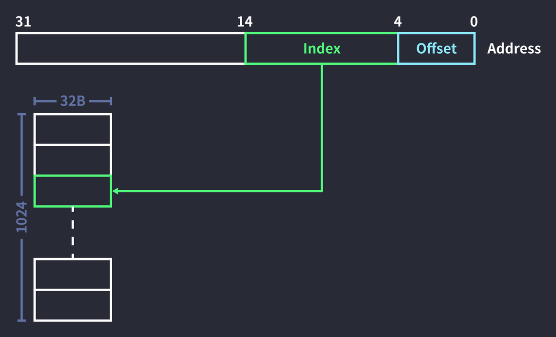
Here, the low 5 bits of the full address are used as the offset, and the next 10 bits are used as the index to access a block. The index is 10 bits because representing every index of $2^n$ blocks requires $log{_2}\text{blocks}$ bits. Since there are $2^{10} = 1024$ blocks here, $log{_2} 1024 = 10$ , so 10 bits are used as index bits. (I’ll explain the offset bits below.)

But doing only this leaves too great a risk that different pieces of data will share the same index.

Tag Matching

To reduce index collisions, part of the address is used as a tag. Suppose there are 1,024 blocks, a block size of 32 bytes, and we access the 32-bit address 0x000c14B8:

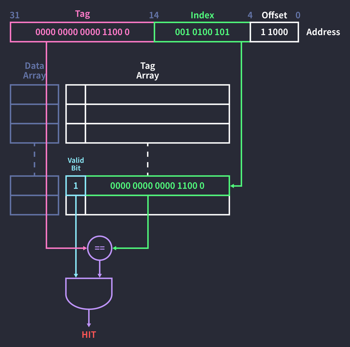
Accessing data through an index and a tag.

First, access the field of the tag array that corresponds to the index (0010100101).
Next, check the valid bit of that tag field.
If the valid bit is 1, compare whether the tag field (00000000000011000) and the address’s tag (00000000000011000) are equal.
AND the comparison result (true, 1) with the valid bit (1).

A valid bit of 1 means a correct value exists in that block. The tag field and the address’s tag match, and the valid bit is 1, so the result of the example above is a hit. On a hit, the data at that index is referenced from the data array. (For reference, the data array and the tag array are both hardware too.)

If the valid bit is 0, it means the block has no value or an invalid one, so a miss occurs. In that case, the address’s tag is written into the tag field, the value requested from a higher-level cache or memory is fetched and written into the data field, and the valid bit is changed to 1.

Even if the valid bit is 1, a miss occurs when the tag doesn’t match. In that case, how it’s handled depends on the replacement policy. If you use the FIFO (First-In First-Out) policy, where the data that came in first is replaced first, the existing block is always replaced. The tag array’s field is changed to the address’s tag, and the data requested from a higher-level cache or memory is fetched to replace the value in the data field with the new data. (In practice, not only the requested data but also the data around it is fetched.) The existing data is pushed up to the higher-level cache.

The reason the upper 15 bits of the address are used as tag bits is that the number of tag bits is determined by $\text{Address bits} - (\log{_2}\text{Block size} + \text{Index bits})$ . In this case, $32 - (5 + 10) = 17$ bits are used as tag bits, and the remaining 5 bits are used as offset bits.

Tag Overhead

Adding the tag array means more space is needed. But a “32KB cache” still means a cache that can store 32KB of data. That’s because the space for tags is treated as overhead, independent of the block size.

Let’s work out the tag overhead of a 32KB cache made up of 1,024 32B blocks:

\begin{aligned} 17 \text{bit tag} + 1 \text{bit valid} &= 18 \text{bit} \\ 18 \text{bit} \times 1024 = 18 \text{Kb tags} &= 2.25 \text{KB} \end{aligned}

In other words, a tag overhead of 7% arises.

There’s a time cost as well as a space cost. Because you access the tag array to check for a hit and only then access the data array to fetch the data, hit latency ends up increasing.

So the two steps are run in parallel: while the tag array is being checked for a hit, the data array is accessed ahead of time. This reduces hit latency, but you have to accept the wasted resources when a miss occurs.

Associative Cache

When two different addresses have the same index, a collision occurs, and a block is replaced according to the replacement policy. But changing the cache’s contents on every collision leads to more misses and can cause the ping-pong problem, where the contents of a single slot are swapped out endlessly.

This problem can be improved by creating multiple tag arrays and data arrays. In other words, the index ends up pointing to several blocks. Classifying caches by the number of blocks an index points to gives the following:

Direct mapped: The index points to a single slot. Fast to process, but collisions happen often.
Fully associative: The index points to every slot. Few collisions, but slow because every block has to be searched.
Set associative: The index points to two or more slots. This is called an n-way set associative cache.

The pros and cons of both direct mapped and fully associative caches are extreme, so a set associative cache is usually used.

Set Associative Cache Organization

Let’s take a quick look at how a 2-way set associative cache works:

How a 2-way set associative cache works.

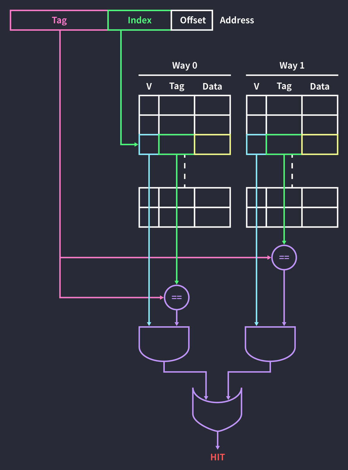
Accessing a block through the address’s index is the same as in the direct mapped cache we’ve seen so far. The difference is that there are two ways, so checking whether the data is cached means checking both blocks, not just one. Finally, ORing the results of the two ways gives the final result. If a miss occurs in every way, data is written into one of the two blocks according to the replacement policy.

Compared with a direct mapped cache, this raises hit latency in exchange for reducing the chance of collisions.

Concrete Example

Suppose we have an 8-byte 2-way cache made up of 2-byte cache blocks, and we’re given a 4-bit address.

Referencing 0001.

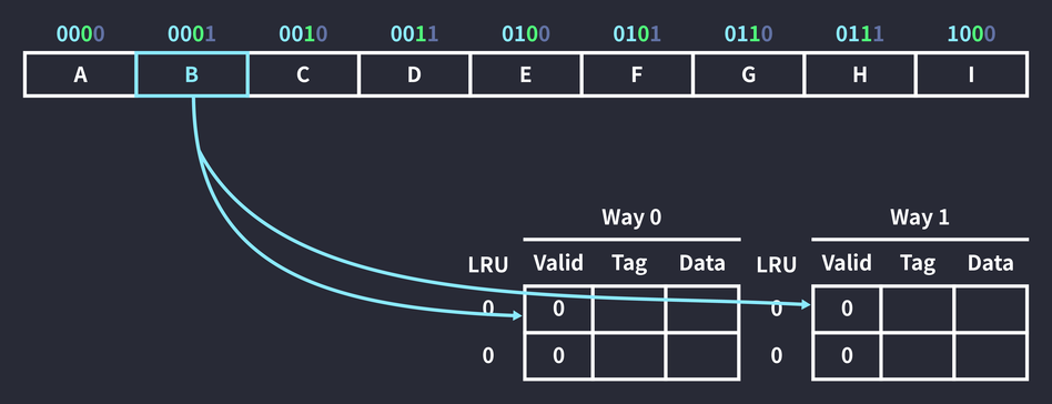
An instruction that references memory address 0001 runs. The index bits are $\log{_2} 2 = 1$ , and the tag bits are $4 - (log{_2} 2 + 1) = 2$ . Finally, the offset bit comes to 1. So the index of address 0001 is 0 and its tag is 00. This means the data at that memory location can be cached in one of the two slots whose index is 0.

Caching 0001 and 0010.

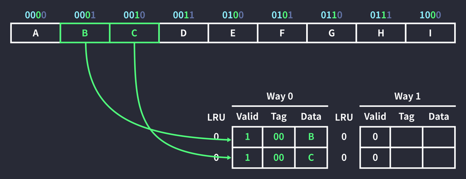
Since the block in Way 0 is empty, the data was stored in the block with index 0 in Way 0. Address 0010 was cached at the same time, because to raise the cache hit rate, memory is fetched a full cache block (2B) at a time. (This takes advantage of spatial locality.) Here, 0010, the space next to the referenced data (0001), was cached along with it.

Referencing 0101.

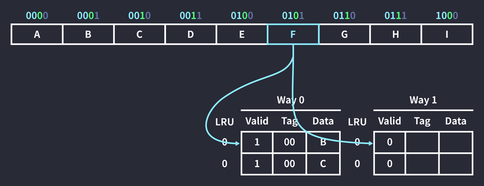
An instruction that references memory address 0101 runs. Again, it can go into either of the two slots whose index is 0.

Caching 0101 and 0110.

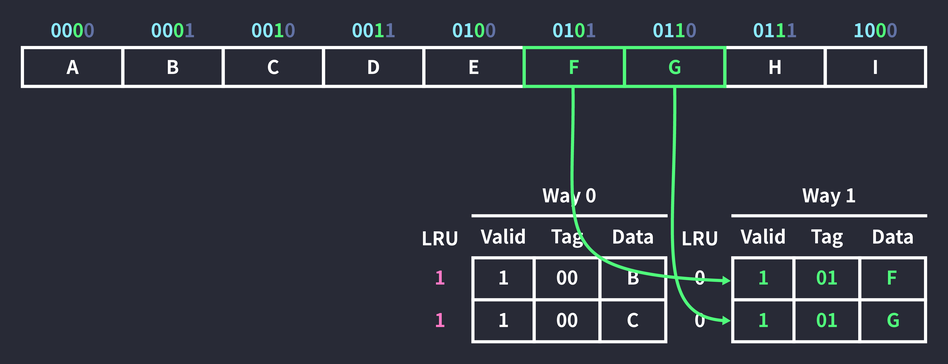
But since the block with index 0 in Way 0 already holds data, the new data is cached in Way 1, which is empty. Once again, the neighboring 0110 data was cached along with it. The LRU (Least Recently Used) values of the two blocks in Way 0 also went up. LRU is a policy that replaces less recently used data first, and it’s also used in the operating system’s process scheduling and in page replacement algorithms. A higher LRU value means a block is more likely to be replaced first when a cache miss occurs.

Referencing 1000. A miss occurs.

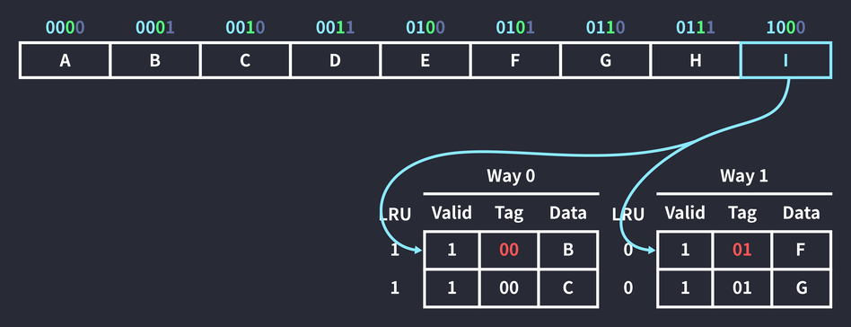
Next, an instruction that references memory address 1000 runs. Both blocks with index 0 were checked, but there was no data with tag 10, so a cache miss occurred.

Caching 0111 and 1000.

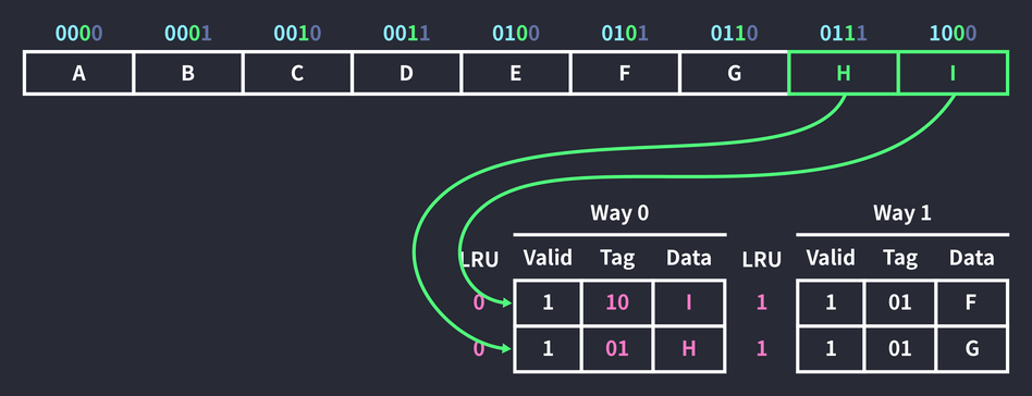
So cached data is replaced. Of the two slots, the Way 0 block has the higher LRU value, so the first block in Way 0 was replaced, and since it was referenced, its LRU value was reset to 0. (The LRU value is also reset on a cache hit.) By the same principle, the data in 0111, the space next to the referenced data, was cached as well. The two blocks in Way 1 weren’t referenced this time, so their LRU values went up.

Handling Cache Writes

When the operation is a write rather than a read, and the address whose data will change is already cached (a write hit), the data in the cache block is updated instead of the data in memory. Now a question arises: “When should the data updated in the cache be written to memory?” There are two write policies.

One is the write-through approach: every time data is written to the cache, the data in memory is updated as well. This generates a lot of traffic, but it keeps the data in memory and the cache identical.

The other is the write-back approach, which updates the data in memory only when a block is replaced. To check whether the data has changed, a dirty bit has to be added to each cache block, set to 1 when the data changes. Later, when that block is replaced, the data in memory is updated if the dirty bit is 1.

If the address whose data will change isn’t cached (a write miss), the write-allocate approach is used. Obviously enough, when a miss occurs the data is cached. Skipping write-allocate would save resources for the moment, but it wouldn’t achieve the cache’s purpose.

Software Restructuring

So far we’ve looked at cache structure and behavior at the low level, but you can also improve cache efficiency at the code level. Look at the following nested loop:

for (i = 0; i < columns; i += 1) {
  for (j = 0; j < rows; j += 1) {
    arr[j][i] = pow(arr[j][i]);
  }
}

This loop squares every element of a 2D array. It looks fine, but in terms of spatial locality it’s inefficient code, because the elements of array arr are stored consecutively in memory while the access isn’t sequential.

0          4          8          12         16         20         24
+----------+----------+----------+----------+----------+----------+
|  [0, 0]  |  [0, 1]  |  [0, 2]  |  [1, 0]  |  [1, 1]  |  [1, 2]  |
+----------+----------+----------+----------+----------+----------+

i = 0, j = 0: accesses the first slot, [0, 0].
i = 0, j = 1: accesses the fourth slot, [1, 0].
i = 1, j = 0: accesses the second slot, [0, 1].

As you can see, the access jumps all over memory. So, as in the code below, the outer loop should iterate over rows and the inner loop over columns.

for (i = 0; i < rows; i += 1) {
  for (j = 0; j < columns; j += 1) {
    arr[i][j] = pow(arr[i][j]);
  }
}

There’s a similar example that takes advantage of temporal locality. Look at the following loop:

for (i = 0; i < n; i += 1) {
  for (j = 0; j < len; j += 1) {
    arr[j] = pow(arr[j]);
  }
}

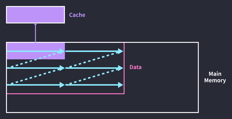
This is a nested loop that repeats the operation of squaring every element of array arr n times. As written, the code gives no guarantee that after caching data, the next access will reach the cached data. If the full dataset is larger than the cache, iterating over the array would look like the figure below.

The cache block is replaced before the cached data is accessed again.

The first half of the loop caches data, but by the time the loop ends, the cache has been overwritten with the data accessed in the second half. So on the second pass, the first-half data has to be cached again. The entire cache block gets replaced before the cached data is ever accessed again. You can solve this by breaking the array’s iteration cycle into chunks the size of the cache.

Accessing the cached data continuously.

The number of loop iterations went up, but the cache hit rate got higher. Through the third pass it processes only the first-half data, and after that only the second-half data. Implemented in code, it becomes a triple loop(!):

for (i = 0; i < len; i += CACHE_SIZE) {
  for (j = 0; j < n; j += 1) {
    for (k = 0; k < CACHE_SIZE; k += 1) {
      arr[i + k] = pow(arr[i + k]);
    }
  }
}

Of course, these days the compiler takes care of all this optimization, so application developers don’t need to worry about this kind of thing. It’s probably enough to know that “code can be optimized like this at the low level.”

References

David Patterson, John Hennenssy, “Computer Organization and Design 5th Ed.”, MK, 2014.
Abraham Silberschatz, Peter Galvin, Greg Gagne, “Operating System Concepts 9th Ed.”, Wiley, 2014.
K. G. Smitha, “Para Cache Simulator”.